4  Deep Learning Models Overview

The goal of this lecture is to understand the core principles and architectures of deep learning models. We will learn how deep learning extends traditional machine learning through multi-layer neural networks, explore the mathematical foundation behind neural computations, and understand how training and optimization methods such as gradient descent enable models to learn complex patterns from data.

Objectives

1. Describe how Deep Learning (DL) fits within the broader field of Machine Learning (ML) and Artificial Intelligence (AI).
2. Explain the structure and mathematical operations of a neural network, including layers, weights, biases, and activations.
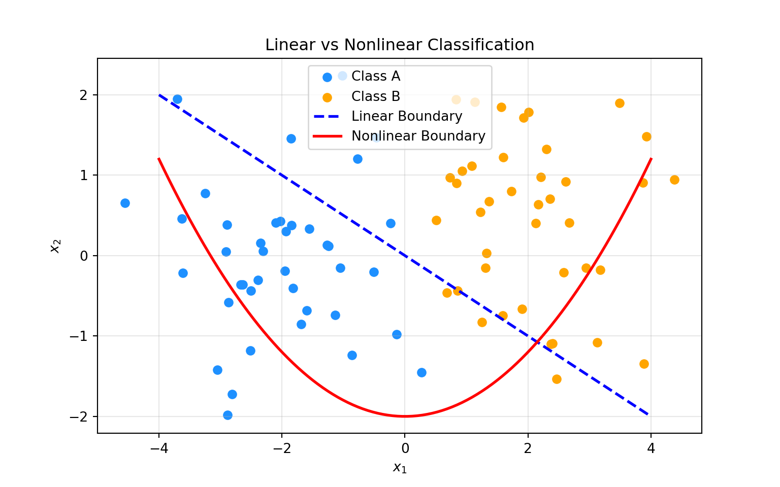
3. Distinguish between linear and non-linear models, and understand how non-linearity enables complex decision boundaries.
4. Apply concepts of activation functions such as sigmoid, tanh, and ReLU, and interpret their mathematical properties.
5. Understand the training process of deep neural networks using gradient descent and backpropagation.
6. Discuss common problems such as overfitting, vanishing gradients, and how regularization and normalization techniques mitigate them.
7. Identify the structure and purpose of key architectures including Convolutional Neural Networks (CNNs), Recurrent Neural Networks (RNNs), and Transformers.

Reading materials

• CS231n: Convolutional Neural Networks for Visual Recognition – Stanford University
• Goodfellow, Bengio & Courville (2016) – Deep Learning, MIT Press, Chapters 6–8
• Hung-Yi Lee – Deep Learning Tutorial
• Ismini Lourentzou – Introduction to Deep Learning
• Sebastian Ruder (2016) – An Overview of Gradient Descent Optimization Algorithms

4.1 Machine Learning Basics

Machine learning enables computers to learn patterns from data without explicit programming. The goal of an ML model is to find a mapping function:

Machine learning aims to learn a function \(f_\theta\) that maps inputs \(x\) to outputs \(y\):

\[ f_\theta : X \rightarrow Y, \]

where \(\theta\) represents model parameters (weights and biases).
The learning objective is to minimize the expected loss:

\[ \theta^* = \arg\min_\theta \, \mathbb{E}_{(x, y) \sim D}[L(y, f_\theta(x))]. \]

4.2 Types of Machine Learning

4.2.1 Supervised Learning

Learns from labeled pairs \((x_i, y_i)\) to predict \(\hat{y_i}\).

• Regression: \(y_i = f_\theta(x_i) + \varepsilon_i\)
• Classification: \(P(y=1|x) = \frac{1}{1 + e^{-(\beta_0 + \beta_1x)}}\)

4.2.2 Unsupervised Learning

Finds structure in unlabeled data \(\{x_i\}\).

• Clustering: \[ \min_{\{C_k\}} \sum_{k=1}^K \sum_{x_i \in C_k} \|x_i - \mu_k\|^2 \]
• PCA: \[ W^* = \arg\max_W \det(W^\top S W) \]

4.2.3 Reinforcement Learning

Learns a policy \(\pi(a|s)\) that maximizes reward:

\[ J(\pi) = \mathbb{E}\left[\sum_{t=0}^{T}\gamma^t r_t\right]. \]

4.3 3. Linear vs Nonlinear Models

A linear classifier defines a boundary:

\[ \mathbf{w}^\top \mathbf{x} + b = 0. \]

A nonlinear classifier maps data to a transformed space \(\phi(x)\):

\[ f(x) = \mathbf{w}^\top \phi(x) + b. \]

Neural networks learn these nonlinear transformations automatically through layers of activations.

import matplotlib.pyplot as plt
import numpy as np

# Generate synthetic data
np.random.seed(0)
X1 = np.random.randn(40, 2) + np.array([-2, 0])
X2 = np.random.randn(40, 2) + np.array([2, 0])

# Plot points
plt.scatter(X1[:, 0], X1[:, 1], color="dodgerblue", label="Class A")
plt.scatter(X2[:, 0], X2[:, 1], color="orange", label="Class B")

# Linear boundary
x_vals = np.linspace(-4, 4, 100)
plt.plot(x_vals, -0.5 * x_vals, 'b--', lw=2, label="Linear Boundary")

# Nonlinear boundary (quadratic)
plt.plot(x_vals, 0.2 * x_vals**2 - 2, 'r-', lw=2, label="Nonlinear Boundary")

plt.title("Linear vs Nonlinear Classification")
plt.xlabel("$x_1$")
plt.ylabel("$x_2$")
plt.legend()
plt.grid(alpha=0.3)
plt.show()

4.4 Structure of Neural Networks

Each neuron performs a linear combination followed by a nonlinear transformation:

\[ z = \mathbf{w}^\top \mathbf{x} + b, \quad a = \sigma(z) \]

For a deep network with \(L\) layers:

\[ \begin{aligned} a^{(1)} &= \sigma(W^{(1)}x + b^{(1)}) \\ a^{(2)} &= \sigma(W^{(2)}a^{(1)} + b^{(2)}) \\ &\vdots \\ \hat{y} &= \sigma(W^{(L)}a^{(L-1)} + b^{(L)}) \end{aligned} \]

4.5 Activation Functions

Function	Formula	Range	Notes
Sigmoid	\(\sigma(x) = \frac{1}{1 + e^{-x}}\)	(0, 1)	Saturates, causes vanishing gradients
Tanh	\(\tanh(x) = \frac{e^x - e^{-x}}{e^x + e^{-x}}\)	(-1, 1)	Zero-centered
ReLU	\(\text{ReLU}(x) = \max(0, x)\)	[0, ∞)	Fast and sparse
Leaky ReLU	\(\text{LeakyReLU}(x) = \max(\alpha x, x)\)	(-∞, ∞)	Fixes “dying ReLU”
Linear	\(f(x) = cx\)	(-∞, ∞)	Used in regression

4.6 Loss Functions

To train a network, we minimize a loss function \(L(y, \hat{y})\):

• Mean Squared Error (MSE): \[ L = \frac{1}{N}\sum_{i=1}^{N}(y_i - \hat{y}_i)^2 \]
• Cross-Entropy Loss: \[ L = -\sum_i y_i \log(\hat{y}_i) \]

4.7 Gradient Descent

Model parameters are updated iteratively:

\[ \theta_{t+1} = \theta_t - \eta \nabla_\theta L(\theta_t), \]

where \(\eta\) is the learning rate.

4.7.1 Mini-batch Gradient Descent

\[ \theta_{t+1} = \theta_t - \frac{\eta}{m} \sum_{i=1}^{m}\nabla_\theta L_i(\theta_t) \]

Balances speed and stability in updates.

4.8 Momentum and Learning Rate Schedules

Add momentum to accelerate convergence:

\[ v_t = \beta v_{t-1} + (1 - \beta)\nabla_\theta L(\theta_t), \quad \theta_{t+1} = \theta_t - \eta v_t \]

Learning rate schedules:

• Step decay: \(\eta_t = \eta_0 \gamma^{\lfloor t/s \rfloor}\)
• Exponential decay: \(\eta_t = \eta_0 e^{-\lambda t}\)
• Cosine annealing: \(\eta_t = \eta_0 \frac{1}{2}(1 + \cos(\pi t/T))\)

4.9 Vanishing and Exploding Gradients

Gradients may vanish or explode when propagated through many layers:

\[ \frac{\partial L}{\partial W^{(l)}} \propto \prod_{i>l} \frac{\partial a^{(i)}}{\partial z^{(i)}} \]

Solutions: - ReLU activations - Batch normalization - Gradient clipping - LSTM gates in RNNs

4.10 Regularization for Generalization

4.10.1 Weight Decay

\[ L' = L + \lambda \|W\|_2^2 \]

4.10.2 Dropout

\[ a_i' = a_i \cdot r_i, \quad r_i \sim \text{Bernoulli}(1 - p) \]

4.10.3 Early Stopping

Stop when validation loss no longer improves.

4.10.4 Batch Normalization

\[ \hat{x} = \frac{x - \mu_B}{\sqrt{\sigma_B^2 + \epsilon}}, \quad y = \gamma \hat{x} + \beta \]

4.11 Convolutional Neural Networks (CNNs)

Convolution extracts local spatial features:

\[ Y(i, j) = \sum_m \sum_n X(i + m, j + n) K(m, n) \]

Pooling reduces spatial dimension:

• Max Pooling: \(y = \max(x_1, \dots, x_n)\)
  
• Average Pooling: \(y = \frac{1}{n}\sum_i x_i\)

4.12 Residual Networks (ResNets)

Residual connections help train very deep networks:

\[ y = F(x) + x \]

The network learns the residual mapping \(F(x) = H(x) - x\), stabilizing gradients across hundreds of layers.

4.13 Recurrent Neural Networks (RNNs)

Sequential models update a hidden state over time:

\[ h_t = f(W_h h_{t-1} + W_x x_t + b) \]

4.13.1 Long Short-Term Memory (LSTM)

\[ \begin{aligned} i_t &= \sigma(W_i x_t + U_i h_{t-1} + b_i) \\ f_t &= \sigma(W_f x_t + U_f h_{t-1} + b_f) \\ o_t &= \sigma(W_o x_t + U_o h_{t-1} + b_o) \\ c_t &= f_t \odot c_{t-1} + i_t \odot \tanh(W_c x_t + U_c h_{t-1} + b_c) \\ h_t &= o_t \odot \tanh(c_t) \end{aligned} \]

4.14 Transformer Networks

Self-attention replaces recurrence, allowing parallel computation.

\[ \text{Attention}(Q, K, V) = \text{softmax}\left(\frac{QK^\top}{\sqrt{d_k}}\right)V \]

Multiple heads attend to different relationships:

\[ \text{MultiHead}(Q, K, V) = \text{Concat}(head_1, \ldots, head_h) W^O \]

Transformers power modern large language models such as GPT and BERT.

4.15 Summary

Deep learning combines principles of linear algebra, calculus, and probability to learn from massive datasets.

\[ \text{Forward Pass: } y = f_\theta(x), \quad \text{Backward Pass: } \theta \leftarrow \theta - \eta \nabla_\theta L \]

From perceptrons to transformers, every model refines this foundation — learning richer representations through mathematics and computation.