Attaching package: 'dplyr'The following objects are masked from 'package:stats':
filter, lagThe following objects are masked from 'package:base':
intersect, setdiff, setequal, union
Attaching package: 'dplyr'The following objects are masked from 'package:stats':
filter, lagThe following objects are masked from 'package:base':
intersect, setdiff, setequal, unionWe can often hypothesize that the standard deviation of residuals in the model \[ y_i=\beta_0+\beta_1x_i+\varepsilon_i \tag{1}\] is proportional to the predictor \(X\), so \[ \mathrm{var}(\varepsilon_i)=k^2x^2_i, \;\; k>0. \]
In the weighted least squares (WLS) method, we can stabilize the variance by dividing both sides of Equation 1 by \(x_i\): \[ \frac{y_i}{x_i}=\frac{\beta_0}{x_i}+\beta_1+\frac{\varepsilon_i}{x_i}, \tag{2}\] then \(\mathrm{var}\left(\frac{\varepsilon_i}{x_i}\right)=k^2\), i.e., it is now stabilized.
Consider a simulated example of a linear model \(y=3-2x\) with noise, which is a function of \(x\).
set.seed(111)
k = 0.5
n = 100
x <- rnorm(n, 0, 5)
y <- 3 - 2 * x + rnorm(n, 0, k*x^2)
The coefficients estimated using ordinary least squares (OLS):
fit_ols <- lm(y ~ x)
summary(fit_ols)
Call:
lm(formula = y ~ x)

Residuals:
   Min     1Q Median     3Q    Max
-47.41  -8.01  -2.32   1.58 286.47

Coefficients:
            Estimate Std. Error t value Pr(>|t|)
(Intercept)    6.131      3.402    1.80    0.075 .
x             -3.571      0.639   -5.59    2e-07 ***
---
Signif. codes:  0 '***' 0.001 '**' 0.01 '*' 0.05 '.' 0.1 ' ' 1

Residual standard error: 34 on 98 degrees of freedom
Multiple R-squared:  0.242, Adjusted R-squared:  0.234
F-statistic: 31.3 on 1 and 98 DF,  p-value: 2.04e-07
Based on Figure 1, the OLS assumption of homoskedasticity is violated, because the observations deviate farther from the regression line at its ends (i.e., the variability of regression residuals is higher at the low and high values of the predictor).
p1 <- ggplot(data.frame(x, y), aes(x = x, y = y)) +
    geom_abline(intercept = 3, slope = -2, col = "gray50", lwd = 1.5) +
    geom_abline(intercept = fit_ols$coefficients[1],
                slope = fit_ols$coefficients[2], lty = 2) +
    geom_point()
p2 <- ggplot(data.frame(x, y), aes(x = x, y = rstandard(fit_ols))) +
    geom_hline(yintercept = 0, col = "gray50") +
    geom_point() +
    xlab("x") +
    ylab("Standardized residuals")
p1 + p2 +
    plot_annotation(tag_levels = 'A')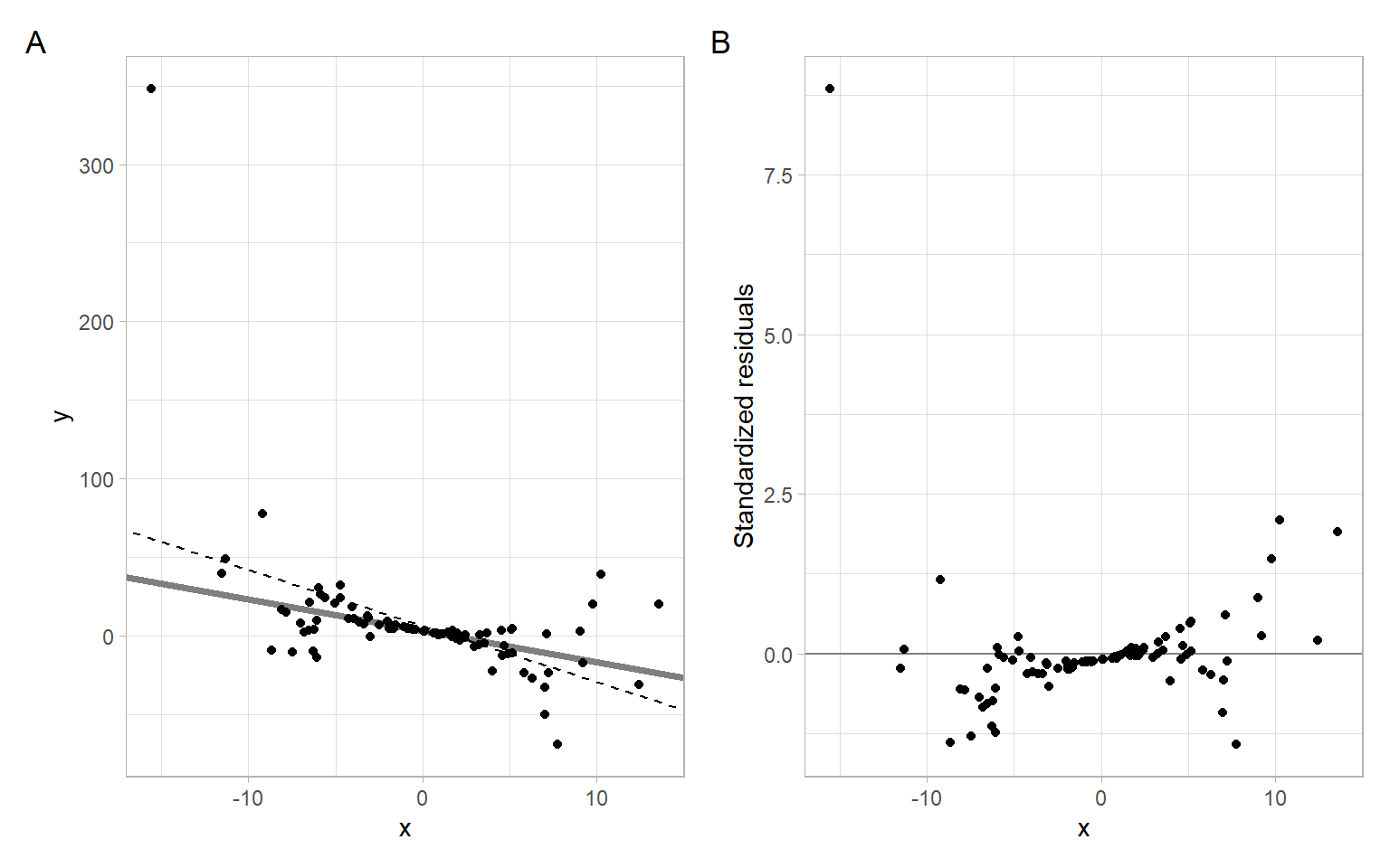
To stabilize the variance ‘manually,’ transform the variables according to Equation 2 and refit the model:
Y.t <- y/x
X.t <- 1/x
fit_wls <- lm(Y.t ~ X.t)
summary(fit_wls)
Call:
lm(formula = Y.t ~ X.t)

Residuals:
    Min      1Q  Median      3Q     Max
-20.021  -0.635   0.251   1.322   5.676

Coefficients:
            Estimate Std. Error t value Pr(>|t|)
(Intercept)   -2.154      0.293   -7.36  5.7e-11 ***
X.t            3.008      0.168   17.95  < 2e-16 ***
---
Signif. codes:  0 '***' 0.001 '**' 0.01 '*' 0.05 '.' 0.1 ' ' 1

Residual standard error: 2.9 on 98 degrees of freedom
Multiple R-squared:  0.767, Adjusted R-squared:  0.764
F-statistic:  322 on 1 and 98 DF,  p-value: <2e-16
Check Equation 2 to see the correspondence of the coefficients, see the results in Figure 2.
p1 <- ggplot(data.frame(x, y), aes(x = x, y = y)) +
    geom_abline(intercept = 3, slope = -2, col = "gray50", lwd = 1.5) +
    geom_abline(intercept = fit_wls$coefficients[2],
                slope = fit_wls$coefficients[1], lty = 2) +
    geom_point()
p2 <- ggplot(data.frame(x, y), aes(x = x, y = rstandard(fit_wls))) +
    geom_hline(yintercept = 0, col = "gray50") +
    geom_point() +
    xlab("x") +
    ylab("Standardized residuals")
p1 + p2 +
    plot_annotation(tag_levels = 'A')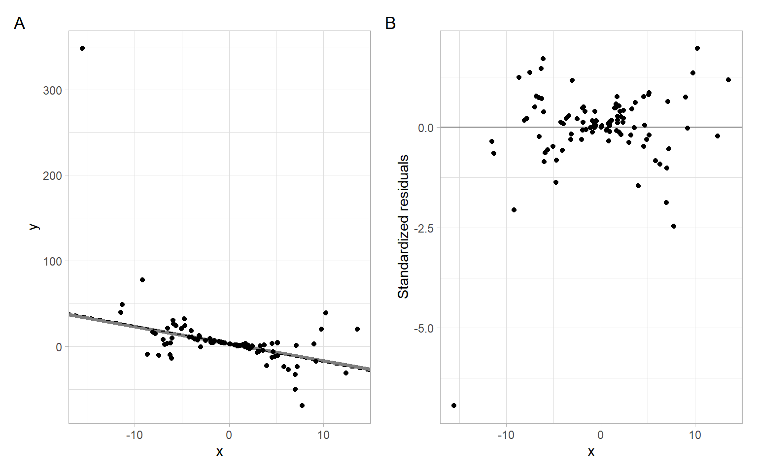
Instead of minimizing the residual sum of squares (using the original or transformed data in Equation 1 and Equation 2), \[ RSS(\beta) = \sum_{i=1}^n(y_i - x_i\beta)^2, \] we minimize the weighted sum of squares, where \(w_i\) are the weights: \[ WSS(\beta; w) = \sum_{i=1}^nw_i(y_i - x_i\beta)^2. \] This includes OLS as the special case when all the weights \(w_i = 1\) (\(i=1,\dots,n\)). In the example above, \(w_i=1/x^2_i\).
In matrix form, \[ \hat{\boldsymbol{\beta}}=(\boldsymbol{X}^{\top}\boldsymbol{W}\boldsymbol{X})^{-1}\boldsymbol{X}^{\top}\boldsymbol{W}\boldsymbol{Y}. \tag{3}\]
To apply Equation 3 in R, specify the argument weights, and remember to take an inverse. Note that the coefficients are now labeled as expected.
fit_wls2 <- lm(y ~ x, weights = 1/x^2)
summary(fit_wls2)
Call:
lm(formula = y ~ x, weights = 1/x^2)

Weighted Residuals:
   Min     1Q Median     3Q    Max
-7.122 -0.842  0.018  1.238 20.021

Coefficients:
            Estimate Std. Error t value Pr(>|t|)
(Intercept)    3.008      0.168   17.95  < 2e-16 ***
x             -2.154      0.293   -7.36  5.7e-11 ***
---
Signif. codes:  0 '***' 0.001 '**' 0.01 '*' 0.05 '.' 0.1 ' ' 1

Residual standard error: 2.9 on 98 degrees of freedom
Multiple R-squared:  0.356, Adjusted R-squared:  0.349
F-statistic: 54.2 on 1 and 98 DF,  p-value: 5.72e-11
@Chatterjee:Hadi:2006 in Chapter 7 consider two more cases for applying WLS, both related to grouping. We skip those cases for now and revisit our data example from ?@sec-regression.
First, use OLS to estimate the simple linear regression exploring dishwasher shipments (DISH) and private residential investments (RES) for several years.
D <- read.delim("data/dish.txt") %>%
    rename(Year = YEAR)
modDish_ols <- lm(DISH ~ RES, data = D)
The plot in Figure 3 indicates that the variance might be decreasing with higher investments.
ggplot(D, aes(x = RES, y = rstandard(modDish_ols))) +
    geom_hline(yintercept = 0, col = "gray50") +
    geom_point() +
    xlab("Residential investments") +
    ylab("Standardized residuals")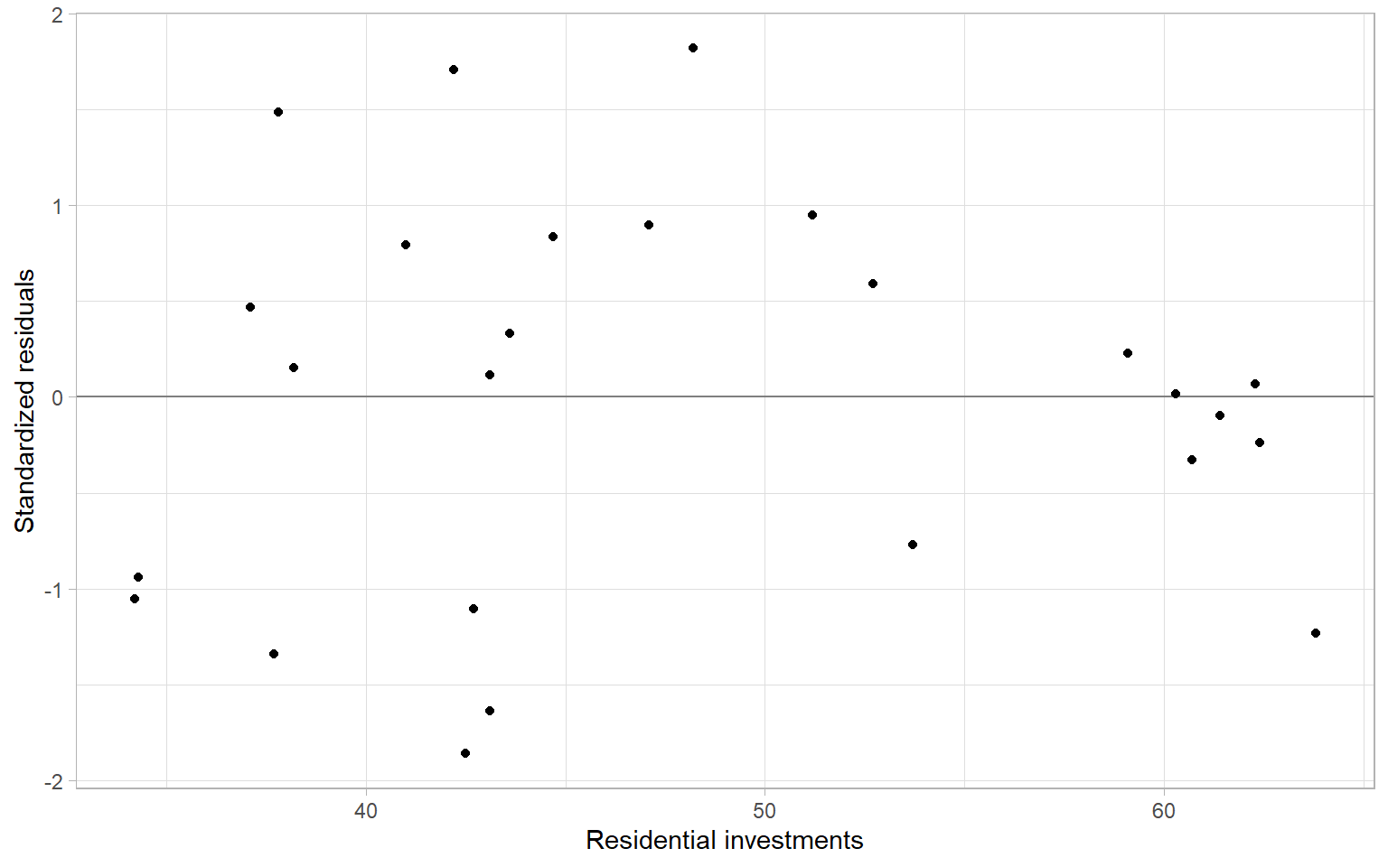
Apply the WLS:
modDish_wls <- lm(DISH ~ RES, data = D, weights = RES^2)In Figure 4 we see minor changes in the slope (better fit?).
p1 <- ggplot(D, aes(x = RES, y = DISH)) +
    geom_abline(intercept = modDish_wls$coefficients[1],
                slope = modDish_wls$coefficients[2], lty = 2) +
    geom_abline(intercept = modDish_ols$coefficients[1],
                slope = modDish_ols$coefficients[2],
                col = "gray50") +
    geom_point() +
    xlab("Residential investments") +
    ylab("Dishwasher shipments")
p2 <- ggplot(D, aes(x = RES, y = rstandard(modDish_wls))) +
    geom_hline(yintercept = 0, col = "gray50") +
    geom_point() +
    xlab("Residential investments") +
    ylab("Standardized residuals")
p1 + p2 +
    plot_annotation(tag_levels = 'A')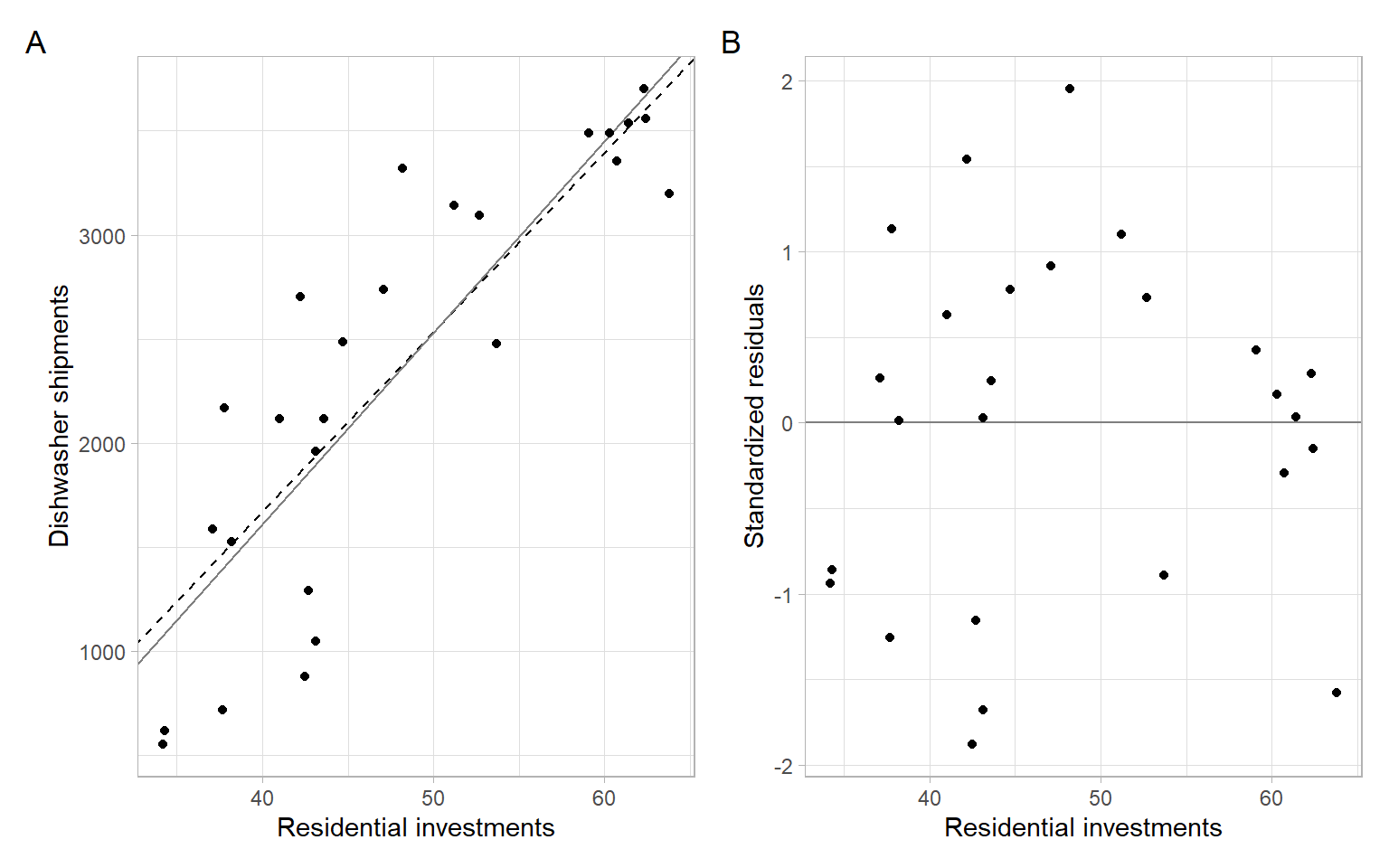
However, the residuals are still autocorrelated, which violates another assumption of the OLS and WLS methods:
lawstat::runs.test(rstandard(modDish_wls))
    Runs Test - Two sided

data:  rstandard(modDish_wls)
Standardized Runs Statistic = -2, p-value = 0.05
See ?@sec-gls on the method of generalized least squares (GLS) that allows accounting for autocorrelation in regression modeling.